
Elliptic Curve Mathematics
Introduction to Elliptic Curves


Introduction to Elliptic Curves
By: Cailyn Yong and Bryan Wee
The elliptic curve has rooted itself into the cryptographic universe, although its math still remains an enigma to the average layman. The history of the curve dates as far back as the 3rd century, when Diophantus of Alexandria explored cubic plane equations in his celebrated work, Arithmetica. But research on elliptic curves only took off in the last few centuries, and has since found importance in fields like public key cryptography, and integer factorization. Today, elliptic curves define the signature schemes that underpin blockchain security.
In this article, we hope to shed some light on curve, and establish the impetus required to develop insight into its use cases.
Basic Math of Elliptic Curves
What is an Elliptic Curve?
An elliptic curve is the set of points that lies on the curve, , together with , the “point at infinity”. The point at infinity is an artificial point on the curve that acts as an ideal point on the projective space of elliptic curves. In other words, it is the point that lies at the ends of all lines parallel to the y-axis.
For practical purposes, we define a rule where for any point on the curve, . With this rule, the set of points on elliptic curves becomes an algebraic closure, meaning any point obtained from applying an algebraic operation on any 2 points on the curve will still belong to the elliptic curve.
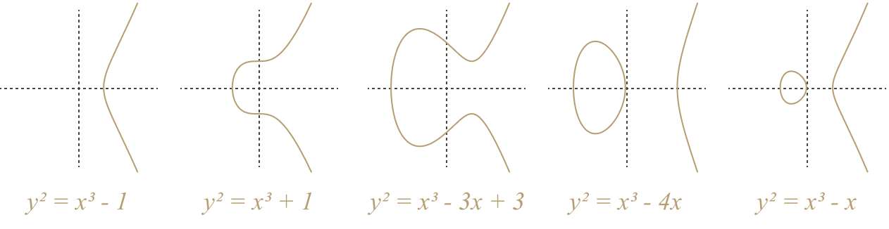
Note that the curve is required to be non-singular, so the discriminant of the curve should not be 0. Geometrically, this means the curve should have no cusps nor self-intersections.
The above cubic equation is called the Weierstrass normal form of elliptic curves. If we look at a few examples of Weierstrass elliptic curves, we can see that there are no cusps nor self-intersecting points.
Elliptic Curve Properties
The points on the curve, along with point addition (which we will define soon), forms an abelian group. In other words, they adhere to the following properties:
Closure under operation: If points and belong to the set of points on the curve, will also belong to that set
Associativity under operation:
Commutativity under operation:
Existence of Identity Element: (note that here is the point at infinity)
Existence of Inverse: Every element has an inverse such that . On elliptic curves, the inverse of is the point symmetric about the x-axis.
Elliptic Curve Point Addition
Point addition in elliptic curves is defined geometrically, and expressed with a simple rule: given any three collinear points on the curve, their sum is always (i.e., the point at infinity). Consequently, . Let us take a look at the graph below to better understand what this looks like.
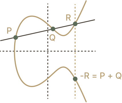
This gives us an intuition on how we can sum two elliptic curve points, and . By connecting the two points and extrapolating the line, a third point is obtained. Reflecting across the x-axis, we find (i.e., the sum).
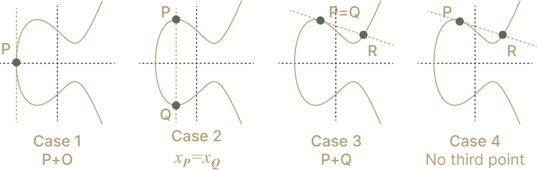
However, this definition does not address a few edge cases:
1. What if ? By definition of , and .
2. What if and are aligned vertically? Since reflects about the x-axis, . Hence, .
3. What if ? This case is termed point doubling, since . In this case, we define the line to be tangent to . Extrapolating this line will give us .
4. What if the line does not intersect a third point? In this case, we can assume that we are in a point doubling scenario (i.e., the third collinear point is either or ). To discern between the two cases, we check the slope of .
If is tangent to , then . Hence, .
Else, is tangent to , and . Hence, .
After defining point addition geometrically, let us try to express it algebraically. If and , how can we express ?
Let us first consider the generic case, .
If
Else if
Else if
Else: let the line be .
•
•
• Then, and .
Next, let us consider the case where (i.e., point doubling).
If
Else:
• The slope
•
•
Elliptic Curve Scalar Multiplication
Other than addition, another operation that comes in handy is scalar multiplication. Recall that is given by extrapolating the line tangent to . This is called point doubling, which is the basis of scalar multiplication. Scalar multiplication is notated like , where is added times onto itself. For instance, if we were to calculate , we could compute .
However, this naive approach to computing can be unduly expensive as that effectively requires . For a 256-bit scalar value (like the ones in Ethereum), this could mean up to point additions, which could take a modern computer approximately years. That is more time than the age of the universe, multiplied by the number of atoms on Earth…
Fortunately, there is a better way. The double-and-add algorithm employs simple memoization to make computation far more efficient. The algorithm is better explained with an example. Take .
Express 113 in powers of 2: .
Recursively pre-compute values of .
Since , we can use our pre-computed values to calculate .
Every natural number can be written as a sum of distinct powers of 2. Just think about how integers are represented in binary!
Computing naively requires 112 point additions. Contrastly, our new approach merely requires 9 point additions.
Generally, to compute , the double-and-add algorithm:
Expresses m in powers of 2.
Recursively pre-compute values of .
Uses pre-computed values to calculate .
Algorithmically, to remove the need to maintain an array of multiples of P, we could interweave steps 2 and 3.
Elliptic Curves over Finite Fields
The elliptic curve we have seen has an infinite number of points. For a computer with finite memory, this might be problematic due to rounding errors and an incapacity to represent an infinite set with a limited number of bits. Thus, elliptic curves must first be restricted to a finite field before they can be computed.
What are Finite Fields?
A field is a set of elements with defined operations for addition, subtraction, multiplication, and division. The defined operations must respect the basic rules of arithmetic. An example of a field is the set of real numbers, where the operations are defined by standard arithmetic.
A finite field, as the name suggests, is a field with a finite set of elements. One example of a finite field is a prime field, a set of integers under modulo , where is a prime number. For prime fields, notated , we define operations to be modulo arithmetic, where we append arithmetic equations with .
For instance, . Results of addition, subtraction, multiplication, and division are all reduced modulo 7. So, for example, .
Restricting the Curve
So far, we have assumed that elliptic curves are defined over real numbers, where and coordinates are real numbers, and arithmetic operations () are the standard ones we are all familiar with. It turns out that elliptic curves can be restricted to other fields, so long as we redefine our arithmetic operations!
To make a curve computable, we want to limit the number of points on the curve to a finite set. This can be achieved by limiting the coordinates to a prime field To do so, we have to redefine arithmetic to be modulo arithmetic. For example, must be intepreted as . Mathematically, the set of points on the curve would be:
Note that elliptic curves over prime fields are still abelian groups, and respect the same properties and formulae as the ones mentioned above. The only difference is that in calculations, standard arithmetic is replaced with modulo arithmetic.
As we have learned, given point and integer , we can compute . Let us now consider the inverse problem. Given points and , what is k such that ?
This problem is called the discrete logarithm problem for elliptic curves and is considered to be computationally hard to solve since it cannot be solved by any known polynomial time algorithm that runs on a computer.
Solving ECDLP
Take two points on an elliptic curve over a finite field, and for some unknown . Let us see how we can compute a valid .
Let be the order of the elliptic curve or the number of unique points on the curve. Consider the sequence
Since addition is closed, each point in the infinite sequence belongs to the elliptic curve. Hence, it should take at most iterations before we find a repeated element in the sequence. This also means that the sequence must be cyclic, where the cycle length is . With that, we can infer the following.
In English, this means if for some unknown , then there exists a valid value of that is less than or equal to . Hence to find , we can use brute force and iterate through to find a valid value of .
There are some well-known algorithms to improve this search. The most popular among them is likely Daniel Shank's Baby-step Giant-step algorithm.
We start by re-expressing .
Let .
Then, can be re-expressed as for some values of and .
We now use Giant-step Baby-step to find and , which consequently gives us .
We first pre-compute all possible values of into a look-up table. This is the baby-step.
Then, we execute the Giant-step. For each possible value of :
• Compute
• Search the result against the look-up table
• If we have found a search hit, we have found valid values of and
Why is this faster? Naive brute force requires at most iterations, but Giant-step Baby-step requires iterations. However, this is still a ridiculous amount of time when is extremely large. For instance, Ethereum's elliptic curve has slightly less than points, which as seen, is an unfathomably large number.
Asymmetric Computational Effort
As we have observed, scalar multiplication of elliptic curve points is easy to compute. Comparatively, the inverse operation is computationally infeasible. This asymmetric relationship is extremely valuable to public key cryptography. Intuitively, by using elliptic curves over finite fields to implement public key cryptography, we can make it easy to infer public key from private key, but not vice versa.
A variant of the discrete logarithm problem also crops up in other cryptographic schemes such as Digital Signature Algorithm (DSA), ElGamal encryption, and Diffie-Hellman key exchange. The difference is that while elliptic curves uses scalar multiplication, the others uses basic modulo arithmetic. In addition, instead of finding in the problem they find such that .
As of today, the discrete logarithm problem for elliptic curves is harder to solve compared to that of the other cryptographic schemes. This makes elliptic curve cryptography more secure than its other cousins, where we need fewer bits of to achieve the same level of security. For instance, a 256-bit private key in elliptic curve cryptography is just as secure as a 3072-bit DSA private key.
Conclusion
We have peered into the elliptic curve and glimpsed over its many properties. We have also toyed with elliptic curve operations: point addition and scalar manipulation, and restricted the curve to a finite field. Lastly, we were introduced to the discrete logarithm problem and gained an intuition on why the elliptic curve is useful in public key cryptography.
Next, we dive a little deeper into elliptic curve math and study how the use of projective spaces can make elliptic curve arithmetic even more efficient...
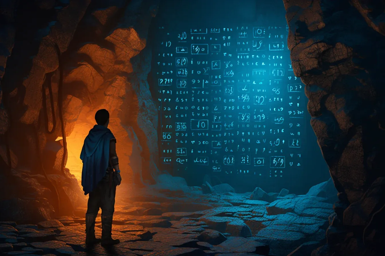
What strange markings, what do they mean?