Projective Coordinates in Elliptic Curves

By: Cailyn Yong and Bryan Wee

Previously, we were introduced to elliptic curves and point operations. So far, the elliptic curves we have seen are represented in the affine space, where points can be represented as $(x,y)$ coordinates. Affine group operations, as we will soon see, are costly as they require field divisions. In this article, we will see how projective coordinates can be used to sidestep these costs and achieve greater efficiency.

Since we are concerned with computational efficiency, we will only be studying curves that are restricted to prime fields. Hence, for all equations below, all field arithmetic is modulo arithmetic.

Cost of Affine Coordinates

Let us consider 2 affine coordinates, $P=(x_1,y_1),Q=(x_2,y_2)$, where $P\ne Q$, and recall how point addition is computed.

1. If either point is $O$, then $P+Q$ is given by the other point.

2. Else if $x_1=x_2$, then $P+Q=O$.

3. Else:
   • Let $m=(y_1-y_2)/(x_1-x_2)$
   • Then, $x_3=m^2-x_1-x_2$ and $y_3=m(x_1-x_3)-y_1$

Let us recall how point doubling can be performed as well. To compute $2P=(x_2,y_2)$, where $P=(x_1,y_1)$:

1. If $P=O$ or $y_1=0$, then $2P=O$

2. Else:
   • Let $m=({3x_1}^2+a)/\left(2y_1\right)$
   • Then, $x_2=m^2-2x_1$ and $y_2=m(x_1-x_2)-y_1$
   

Both point addition and doubling require 1 field division, which for prime fields, means modular division. This form of division requires the non-trivial act of finding a modular inverse, making it very expensive.

Projective Coordinates

Costs can be reduced by adopting a new coordinate system that avoids field division entirely. Given an affine coordinate $(x,y)$, we can transform it into a projective coordinate $(X,Y,Z)$ by taking an arbitrary non-zero value $Z$ and assigning $(X,Y,Z)=(xZ,yZ,Z)$.

For instance, $(2,3)$ can be mapped to $(4,6,2)$ or $(8,12,4)$, with $Z=2$ or $Z=4$ respectively. Usually, $z$ is chosen to be $1$ for convenience; affine coordinates $(x,y)$ would be transformed to $(x,y,1)$.

Projecting an entire elliptic curve yields the following curve equation.

$Y^{2}Z=X^3+aX{Z}^2+b{Z}^3$

The diagram below visualizes how a projected curve might look like.

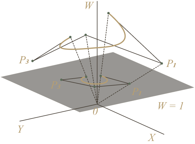
To convert projective coordinates $(X,Y,Z)$ back to affine coordinates $(x,y)$, all we have to do is divide the projective coordinate by $Z$.

$(x,y)=(X/Z,Y/Z)$

With projective coordinates, the formulae for point addition and point doubling require no field division. Take $P=(X_1,Y_1,Z_1)$, $Q=(X_2,Y_2,Z_2)$, and $P\ne Q$. Let us see how we can compute $P+Q=(X_3,Y_3,Z_3)$.

1. If either point is $O$, then $P+Q$ is given by the other point.

2. Else, let:
   • $u=Y_2{Z}_1-Y_1{Z}_2$
   • $v=X_2{Z}_1-X_1{Z}_2$
   • $A=u^2{Z}_1{Z}_2-v^3-2v^2{X}_1{Z}_2$

3. To perform point addition,
   • $X_3=vA$
   • $Y_3=u(v^2{X}_1{Z}_2-A)-v^3{Y}_1{Z}_2$
   • $Z_3=v^3{Z}_1{Z}_2$
   

Next, given $P=(X_1,Y_1,Z_1)$, how can compute $2P=(X_2,Y_2,Z_2)$?

1. Let:
   • $w=a{Z_1}^2+3{X_1}^2$
   • $s=Y_1{Z}_1$
   • $B=X_1{Y}_{1}s$
   • $h=w^2-8B$

2. To perform point doubling:
   • $X_2=2hs$
   • $Y_2=w(4B-h)-8s^2{Y_1}^2$
   • $Z_2=8s^{3}f$
   

Both operations require more addition and multiplication than before, but demand zero divisions! Knowing this, we can much more efficiently manipulate elliptic curve points by:

1. Converting affine coordinates to projective coordinates.

2. Perform the required computation.

3. Converting the results back to affine coordinates. (Only this step requires division)
   

Now, only two field divisions are required for any amount of consecutive point addition and doubling. This, in turn, saves a drastic amount of computation for elliptic curves over finite fields.

Jacobian Coordinates

A modified form of projective coordinates is Jacobian coordinates. For Jacobian coordinates, instead of multiplying $x$ and $y$ with $Z$ like we did in the standard form of projective coordinates, we map affine coordinates $(x,y)$ to $(X,Y,Z)=(x\ast Z^2,y\ast Z^3,Z)$.

Using Jacobian coordinates, elliptic curves adopt the following equation.

$Y^2=X^3+aX{Z}^4+b{Z}^6$

Here is the formula for point addition, assuming $P\ne Q$:

1. If either point is $O$, then $P+Q$ is given by the other point.

2. Else, let:
   • $U_1=X_1{Z_2}^2$ and $U_2=X_2{Z_1}^2$
   • $s=S_1=Y_1{Z_2}^3$ and $S_2=Y_2{Z_1}^3$
   • $H=U_2-U_1$
   • $r=S_2-S_1$
   

3. To perform point addition
   • $X_3=r^2-H^3-2U_1{H}^2$
   • $Y_3=r(U_1{H}^2-X_3)-S_1{H}^3$
   • $Z^3=H{Z}_1{Z}_2$
   

...and the formula for point doubling.

1. If $Y_1=0,$ then $2P=O$.

2. Else, let:
   • $S=4X_1{Y_1}^2$
   • $M=3{X_1}^2+a{Z_1}^4$
   • $T=M^2-2S$
   

3. To perform point doubling:
   • $S=X_2=T$
   • $Y_2=M(S-T)-8{Y_1}^4$
   • $Z_2=2Y_1{Z}_1$
   

Like before, these operations do not require field division. Jacobian coordinates offer a slight edge compared to standard projective coordinates because they trade multiplication for more addition/subtraction which tends to be cheaper.

Jacobian Coordinates ⇌ Affine Coordinates

Each instance of affine point addition/doubling requires one field division. This becomes extremely expensive once we consider consecutive curve operations (e.g., scalar multiplication). On the other hand, Jacobian coordinates demand no field divisions. We can exploit this fact to support affine point manipulation by:

1. Converting affine points to Jacobian points, with $z=1$.

$(x,y)\to (x,y,1)$

2. Performing all necessary operations in Jacobian space.

3. Converting Jacobian points back to affine space. Let $z^{-1}$ be the modular inverse of $z$.

$(x,y,z)\to (x\ast (z^{-1}{)}^2,y\ast \left(z^{-1}{)}^3\right)$

This way, we only require one modular inversion for an arbitrary number of elliptic curve operations, saving a significant amount of computation!

Conclusion

In the previous article, we learned about the elliptic curve and the discrete logarithm problem. We then restricted the curve such that it can be computed by a computer with finite memory.

In this article, we transformed the curve onto a projective space and saw how it optimizes point arithmetic. After much math, we have arrived at a version of elliptic curves that is optimal for computers, and now have the necessary impetus to learn about elliptic curve cryptography.